Exploring the Ansatz Zoo: Heuristics and the Parameter Gap

In our previous post, we hit a theoretical wall.

We calculated that to fully parameterize a unique quantum state for \(N\) qubits, we need:

\[ \text{Params}_{\text{Full}} = 2(2^N) - 2 \]

For a practical \(N=16\) system, this means searching a 130,000-dimensional space. No optimizer can handle that. We need to be smarter. We need a “Heuristic Ansatz”—a circuit template that explores a relevant slice of the Hilbert space using a manageable number of parameters.

1. The Blueprint: n_local

The general strategy for building these templates is the n-local architecture. It consists of alternating layers:

1. Rotation Layers: Single-qubit gates (like \(R_Y, R_Z\)) to explore local states.

2. Entanglement Layers: Multi-qubit gates to mix information.

The term “\(n\)-local” refers to the size of the entangling blocks. The gates act on at most \(n\) qubits at a time. In Qiskit, the n_local() function allows us to build any variation of this structure.

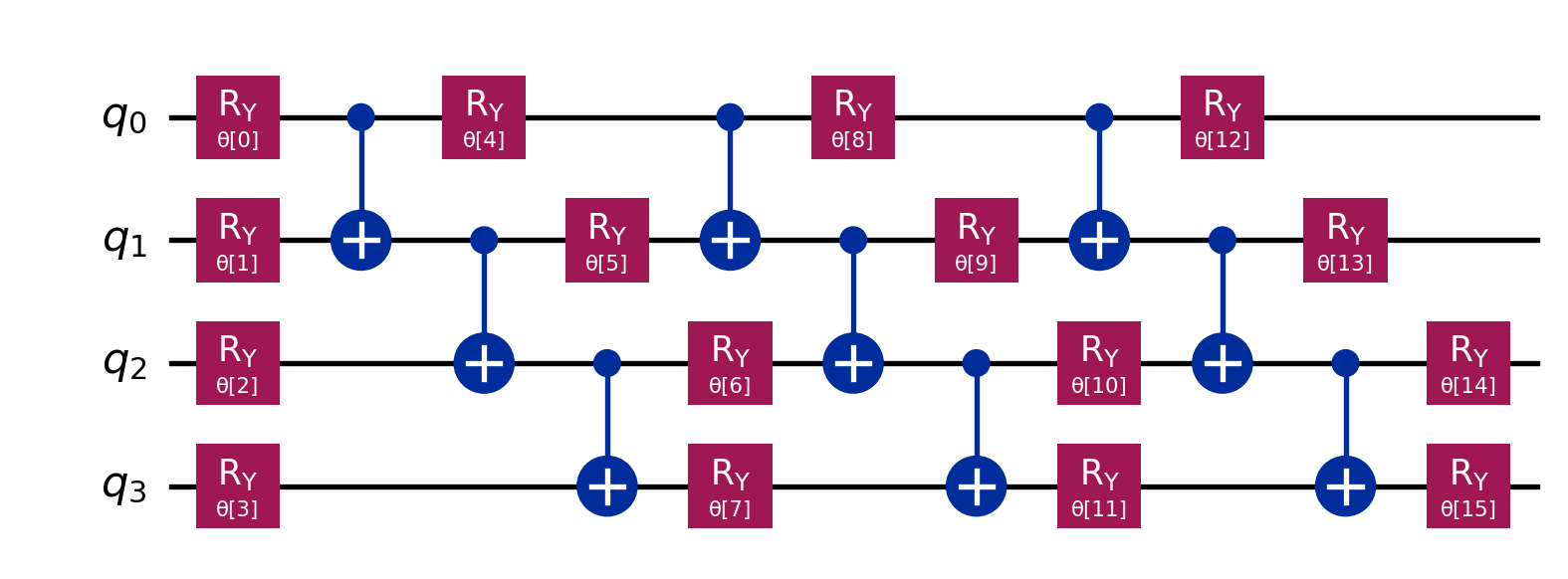
The Road Less Traveled: A 3-Local Example

Most standard ansatzes are 2-local (using pairs of qubits). But to understand why, let’s try to build a 3-local circuit.

We could use a 3-qubit gate, like the Toffoli (CCX), as our entangler.

from qiskit.circuit.library import n_local
from qiskit import QuantumCircuit

# Building a 3-Local Ansatz
# Rotations: RY on every qubit
# Entanglement: CCX (Toffoli) acting on triplets
# We use reps=3 to give it depth
ansatz_3local = n_local(num_qubits=4,
                        rotation_blocks=['ry'],
                        entanglement_blocks='ccx',
                        entanglement=[[0, 1, 2], [1, 2, 3]], # Explicit triplets
                        reps=3,
                        insert_barriers=True)

print(f"3-Local Parameters: {ansatz_3local.num_parameters}")
display(ansatz_3local.draw('mpl'))

3-Local Parameters: 16

Why don’t we use this?

You rarely see 3-local (or 4-local) ansatzes in VQE. There are two main reasons:

1. Hardware Connectivity: Real quantum processors (like IBM’s heavy-hex lattice) only physically connect qubits in pairs. A 3-qubit gate like CCX doesn’t exist natively. The compiler has to break it down into 6+ CNOT gates, making the circuit incredibly deep and noisy.

2. Overkill: We don’t need 3-body gates to create global entanglement. A layer of 2-body CNOTs can spread information across the entire chip in just a few steps (\(O(\log N)\) depth).

2. The Standard: 2-Local

This is why the 2-local structure is the gold standard. It matches the native hardware (CNOT/CZ) and is expressive enough to generate complex states.

While we can use n_local to build them, Qiskit provides optimized helper functions for the two most common patterns: efficient_su2 and real_amplitudes.

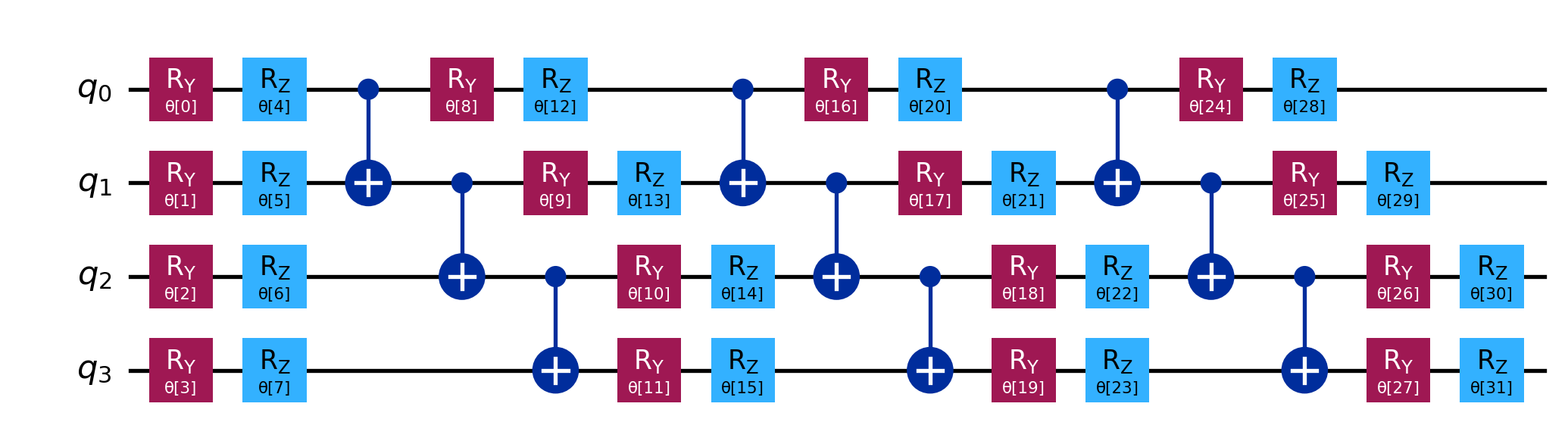
efficient_su2: The Generalist

The efficient_su2 ansatz is designed to be universal for local operations. “SU(2)” refers to the group of operations on a single qubit. This circuit ensures that every qubit can reach any state on its Bloch sphere (using \(R_Y\) and \(R_Z\)) before being entangled.

• Best for: Problems with complex eigenvectors (e.g., non-Hermitian matrices, dynamics).

• Structure: \(R_Y \to R_Z \to \text{CNOT}\).

from qiskit.circuit.library import efficient_su2

# Standard EfficientSU2 with reps=3
# This creates 3 full layers of entanglement
ansatz_su2 = efficient_su2(num_qubits=4,
                           su2_gates=['ry', 'rz'],
                           entanglement='linear',
                           reps=3)

print(f"EfficientSU2 Parameters: {ansatz_su2.num_parameters}")
display(ansatz_su2.draw('mpl'))

EfficientSU2 Parameters: 32

Parameter Count (N=16)

For a 16-qubit system with depth 3: \[ \text{Params} = 2N(d+1) = 2(16)(4) = 128 \] We have reduced the problem from 130,000 variables to 128.

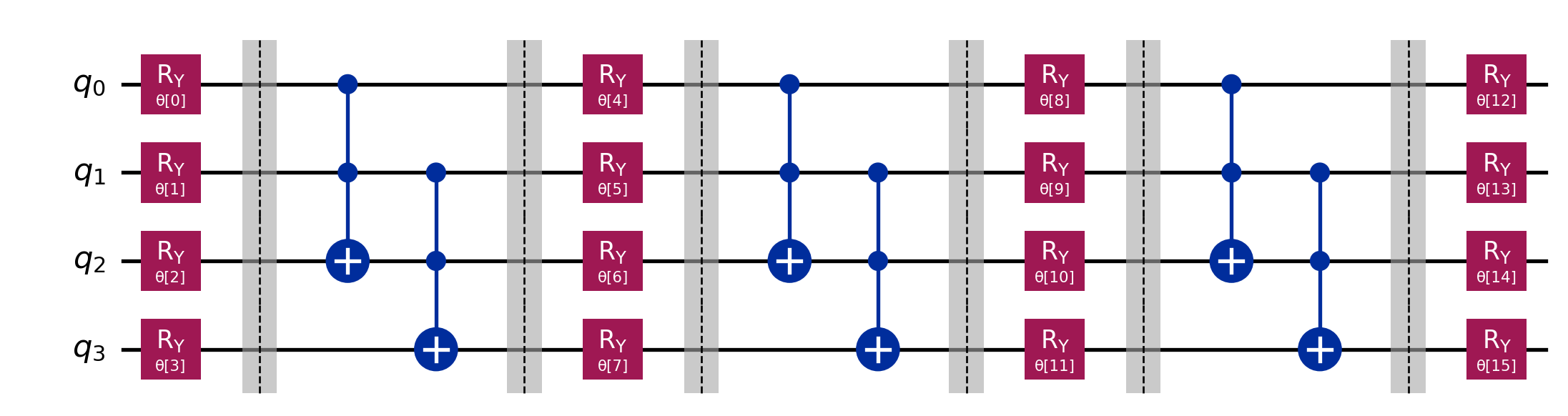
real_amplitudes: The Specialist

For Matrix Diagonalization of real symmetric matrices (our main goal), we know the eigenvectors are real. We can strip out the \(R_Z\) gates. This reduces the parameter count by half, making the optimization easier.

• Best for: Hamiltonian ground states, Machine Learning kernels, Real Symmetric matrices.

• Structure: \(R_Y \to \text{CNOT}\).

from qiskit.circuit.library import real_amplitudes

# Standard RealAmplitudes with reps=3
ansatz_real = real_amplitudes(num_qubits=4,
                              entanglement='linear',
                              reps=3)

print(f"RealAmplitudes Parameters: {ansatz_real.num_parameters}")
display(ansatz_real.draw('mpl'))

RealAmplitudes Parameters: 16

Parameter Count (N=16)

For a 16-qubit system with depth 3: \[ \text{Params} = N(d+1) = 16(4) = 64 \] 64 variables is incredibly lightweight. This gives our optimizer the best possible chance of success.

3. The Goldilocks Choice: Why reps=3?

In all the examples above, we set reps=3. This wasn’t an accident. In heuristic ansatz design, the number of repetitions (depth) is the most critical knob we can turn.

It represents a trade-off between Expressibility and Trainability.

1. Too Shallow (reps=0 or 1): The circuit cannot create enough entanglement. It can only explore “Product States” or very simple correlations. It will likely fail to reach the true ground state.

2. Too Deep (reps=50):

   • Noise: Every additional layer adds CNOT gates. On current hardware, deep circuits accumulate so much noise that the signal becomes garbage.
   • Barren Plateaus: As we add parameters, the high-dimensional optimization landscape becomes increasingly flat. The gradient vanishes, and the optimizer gets stuck.

3. Just Right (reps=3): For many practical problems, 3 layers provide enough entanglement to capture non-trivial correlations, while keeping the parameter count low enough (e.g., 64 vs 1000s) for the classical optimizer to succeed.

4. The Road Not Taken: Specialized Ansatzes

The ansatzes above are “blind”—they don’t know what problem they are solving. They just explore the space.

In some fields, we can do better by building the circuit based on the problem’s physics. We mention them here for completeness, though we won’t use them for general diagonalization.

1. UCCSD (Unitary Coupled Cluster): Used in Chemistry. The gates mimic electron excitations. It is incredibly accurate but produces very deep circuits that are hard to run on near-term hardware.

2. QAOA (Quantum Approximate Optimization Algorithm): Used in Combinatorial Optimization (e.g., MaxCut). The gates alternate between the “Cost Hamiltonian” and a “Mixer,” effectively simulating a time-evolution process.

3. ZZFeatureMap: Used in Machine Learning. This is used to encode classical data into quantum states (kernels) rather than finding ground states.

Why don’t we use them here? Because we are solving a general linear algebra problem. We don’t have the physical intuition of a molecule or a graph to guide us. Therefore, the Hardware Efficient Ansatz (real_amplitudes) is our best general-purpose tool.

5. What’s Next?

We have our Ansatz (real_amplitudes) and our strategy (VQE). But there is a glaring hole in our pipeline.

In all our examples so far, we have been “building” the matrix \(A\) manually in Python (e.g., creating a NumPy array). But if \(N=16\), the matrix has 4 billion entries. We cannot store that in RAM to convert it into a Hamiltonian.

In the next post, we will learn how to represent the matrix implicitly—decomposing a problem into Pauli strings without ever building the full dense matrix.