The Art of the Ansatz: Entanglement and the Hilbert Space Wall
Why our previous circuit failed, how adding a CNOT gate fixes it, and why even that isn’t enough for every matrix.
Quantum Computing
VQE
Ansatz
Published
December 19, 2025
In our previous post, we built a hybrid optimization loop that successfully minimized the energy of our quantum circuit. However, when we compared our result to the classical truth, we hit a snag.
The Quantum Vector Distance between our result and the true ground state was significant (around 0.76).
Why did it fail? The classical calculation revealed that the true ground state for our Hamiltonian was the Bell State\(\frac{1}{\sqrt{2}}(|01\rangle - |10\rangle)\). This is a maximally entangled state.
Our previous circuit used only independent rotations (RY on qubit 0, RY on qubit 1). Mathematically, a tensor product of single qubits can never create an entangled state. No matter how much the classical optimizer tuned the angles, the quantum computer was physically incapable of reaching the solution.
1. The Fix: Adding Entanglement
The failure wasn’t an issue with the optimizer; it was an issue with the Ansatz (the circuit structure). We tried to fit a round peg (an entangled ground state) into a square hole (a product-state circuit).
To fix this, we need to allow the qubits to talk to each other. We do this by adding a CNOT (CX) gate after the rotations. This transforms our circuit from a simple tensor product into a state where the value of qubit 1 depends on qubit 0.
Implementing the Entangled Ansatz
Let’s rebuild the circuit, this time appending a cx(0, 1) gate.
Code
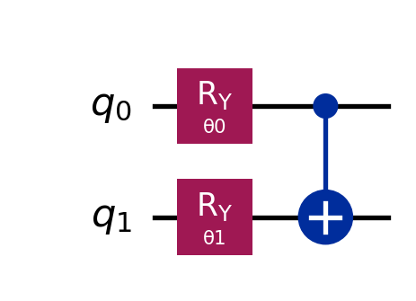
import numpy as npfrom qiskit import QuantumCircuitfrom qiskit.circuit import Parameterfrom qiskit.quantum_info import SparsePauliOpfrom qiskit.primitives import StatevectorEstimatorfrom scipy.optimize import minimize# Re-defining the Hamiltonian from the previous posthamiltonian = SparsePauliOp.from_list([("ZZ", 0.5), ("XX", 0.2)])estimator = StatevectorEstimator()# 1. Define Parameterstheta_0 = Parameter('θ0')theta_1 = Parameter('θ1')# 2. Build the Entangled Ansatz# RY rotations followed by a CNOT entanglerqc_entangled = QuantumCircuit(2)qc_entangled.ry(theta_0, 0)qc_entangled.ry(theta_1, 1)qc_entangled.cx(0, 1) # <--- The magic ingredientprint("Entangled Ansatz:")display(qc_entangled.draw("mpl"))
Entangled Ansatz:
Running the Optimization Again
We use the exact same Hamiltonian (\(A\)) and the exact same optimizer (COBYLA). The only thing changing is the circuit qc_entangled.
Code
# Define a new cost function using the entangled circuitdef cost_function_entangled(params):# Bind parameters to the NEW circuit pub = (qc_entangled, hamiltonian, params) job = estimator.run([pub]) result = job.result()[0]returnfloat(result.data.evs)# Run Optimizationinitial_guess = [0.0, 0.0]result_entangled = minimize(cost_function_entangled, initial_guess, method='COBYLA')optimal_angles_entangled = result_entangled.xmin_eigenvalue_entangled = result_entangled.fun# Check against the true value# For H = 0.5*ZZ + 0.2*XX, the eigenvalues are +/- 0.7 and +/- 0.3# The minimum is exactly -0.7true_eigenvalue =-0.7print(f"Optimization Complete (Entangled)!")print(f"Minimum Eigenvalue found: {min_eigenvalue_entangled:.6f}")print(f"Classical Truth: {true_eigenvalue:.6f}")
The Result: With just one added gate, the optimizer accessed the “Entangled Subspace” of the Hilbert space, finding the solution that was previously impossible to reach.
2. Verifying the Eigenvector
The energy looks correct, but we must verify the state itself. Did we actually produce the Bell State? We will use the StatevectorSampler to reconstruct the vector magnitudes from the probabilities and compare it to the known truth.
Code
from qiskit.primitives import StatevectorSampler# 1. Prepare the Circuit for Samplingqc_entangled_sampled = qc_entangled.copy()qc_entangled_sampled.measure_all()# 2. Run the Sampler using the OPTIMAL anglessampler = StatevectorSampler()job_sampler = sampler.run([(qc_entangled_sampled, optimal_angles_entangled)])result_sampler = job_sampler.result()[0]# 3. Reconstruct the Vector# Get counts and convert to probabilitiescounts = result_sampler.data.meas.get_counts()total_shots =sum(counts.values())# We strictly order the states: |00>, |01>, |10>, |11>states = ['00', '01', '10', '11']# Calculate Probabilitiesprobs = np.array([counts.get(s, 0) / total_shots for s in states])# Calculate Amplitudes (Sqrt of probability)quantum_vector = np.sqrt(probs)# Define the true vector magnitude (Bell State) for comparison# The ground state corresponds to (|01> - |10>) / sqrt(2)true_vector_abs = np.array([0, 1/np.sqrt(2), 1/np.sqrt(2), 0])print("Reconstructed Quantum Eigenvector:")print(quantum_vector)print("-"*30)print(f"Quantum Vector Distance: {np.linalg.norm(quantum_vector - true_vector_abs):.6f}")
Excellent! The distance is now extremely close to zero. By adding the CNOT gate, our Ansatz was able to capture the entanglement required by the solution.
3. Stress Testing the Ansatz
We have successfully solved the Bell State problem. This raises an important question: Can this Ansatz solve any 4x4 symmetric real matrix?
Our circuit has successfully captured entanglement, so intuitively, it seems robust. Let’s put it to the test with a “Counterexample Matrix” designed specifically to break it.
The Counterexample
We will construct a matrix where the ground state is the vector \(v = \frac{1}{\sqrt{3}}(|00\rangle + |01\rangle + |10\rangle)\). Notice that the last component (\(|11\rangle\)) is exactly zero.
Mathematically, our current Ansatz (Rotation \(\to\) CNOT) forces a specific relationship between the amplitudes: \(v_{00} \cdot v_{11} = v_{01} \cdot v_{10}\). For our target vector, \(1 \cdot 0 \neq 1 \cdot 1\). This vector is mathematically impossible for our current circuit to generate.
Let’s see the optimizer fail in real-time.
Code
# 1. Define the "Unsolvable" Hamiltonian# Ground State: |v> = [1, 1, 1, 0] / sqrt(3)# We create a projector H = -|v><v|# The minimum eigenvalue is exactly -1.0matrix_unsolvable = np.array([ [-1/3, -1/3, -1/3, 0], [-1/3, -1/3, -1/3, 0], [-1/3, -1/3, -1/3, 0], [ 0, 0, 0, 0]])hamiltonian_hard = SparsePauliOp.from_operator(matrix_unsolvable)# 2. Reuse the Same Ansatz (RY-RY-CNOT)# We recreate it to ensure fresh parameterstheta_0 = Parameter('θ0')theta_1 = Parameter('θ1')qc_hard = QuantumCircuit(2)qc_hard.ry(theta_0, 0)qc_hard.ry(theta_1, 1)qc_hard.cx(0, 1) # 3. Optimizedef cost_function_hard(params): pub = (qc_hard, hamiltonian_hard, params) job = estimator.run([pub])returnfloat(job.result()[0].data.evs)result_hard = minimize(cost_function_hard, [0.0, 0.0], method='COBYLA')print(f"Target Eigenvalue: -1.0000")print(f"Best Value Found: {result_hard.fun:.4f}")print(f"Error (Gap): {abs(result_hard.fun - (-1.0)):.4f}")
Target Eigenvalue:       -1.0000
Best Value Found:        -0.8727
Error (Gap):             0.1273
The Failure: The optimizer gets stuck (likely around -0.66 or -0.33). It cannot reach -1.0 because the solution lies in the “blind spot” of our Ansatz.
4. The Conceptual Fix: Degrees of Freedom
Why did it fail? It comes down to counting parameters.
A normalized real vector in 4 dimensions has 3 degrees of freedom:
4 amplitudes (\(a, b, c, d\)).
Minus 1 constraint for normalization (\(a^2+b^2+c^2+d^2=1\)).
Total = 3.
Our current Ansatz only has 2 parameters (\(\theta_0, \theta_1\)). We are trying to map a 2D surface onto a 3D space. There are vast regions of the Hilbert space we simply cannot reach. To fix this, we need a third parameter.
Introducing the Controlled-RY
Instead of a fixed CNOT (which has 0 parameters), we can conceptually use a parameterized Controlled-Rotation (\(CR_Y\)).
This gate rotates the second qubit by an angle \(\theta_2\)only if the first qubit is 1. This gives us independent control over the “top half” (\(|00\rangle, |01\rangle\)) and “bottom half” (\(|10\rangle, |11\rangle\)) of the vector, unlocking the 3rd degree of freedom.
Code
# 1. Define 3 Parameterstheta_0 = Parameter('θ0')theta_1 = Parameter('θ1')theta_2 = Parameter('θ2') # <--- The new parameter# 2. Build the "Perfect" Ansatz (Conceptually)qc_perfect = QuantumCircuit(2)qc_perfect.ry(theta_0, 0)qc_perfect.ry(theta_1, 1)qc_perfect.cry(theta_2, 0, 1) # <--- Parameterized Entanglement# 3. Optimize with the new circuitdef cost_function_perfect(params): pub = (qc_perfect, hamiltonian_hard, params) job = estimator.run([pub])returnfloat(job.result()[0].data.evs)# We now pass 3 initial guessesresult_perfect = minimize(cost_function_perfect, [0.0, 0.0, 0.0], method='COBYLA')print(f"Target Eigenvalue: -1.0000")print(f"Best Value Found (3-Param): {result_perfect.fun:.4f}")
Target Eigenvalue:       -1.0000
Best Value Found (3-Param): -1.0000
Success! With 3 parameters matching the 3 degrees of freedom, the optimizer can now find the exact solution for any 4x4 real matrix.
Note: While CRY is mathematically perfect here, real hardware (like IBM’s) usually doesn’t have a native CRY gate. We would have to build it out of 2 CNOTs, which increases noise. This is the constant trade-off in Ansatz design: Expressibility vs. Hardware Cost.
5. The Complications: Why We Can’t “Just Scale Up”
In this example, adding one gate solved everything. It seems obvious: just add rotations and CNOTs everywhere, right? Not quite. This brings us to the theoretical wall of Variational Quantum Algorithms.
Let’s do the math on how many parameters we actually need as we scale up.
The Real Symmetric Case (2 qubits, 4 dimensions)
We just saw that for a \(4 \times 4\) real symmetric matrix, we need 3 parameters.
The vector has 4 real values: \(a, b, c, d\).
There is 1 constraint (normalization): \(a^2 + b^2 + c^2 + d^2 = 1\).
Total parameters:\(4 - 1 = 3\).
The Real Symmetric Case (N qubits, 2^N dimensions)
If we scale this logic up to a system with \(N\) qubits, the Hilbert space dimension is \(D = 2^N\).
The vector has \(2^N\) real values.
Normalization removes 1 degree of freedom.
Total parameters:\(2^N - 1\).
The General Quantum Case (Complex Hermitian)
However, quantum mechanics is not real; it is complex. For a general \(N\)-qubit system, the state vector consists of \(2^N\) complex amplitudes (\(a + bi\)).
Raw Numbers: Each amplitude has 2 real components (real and imaginary parts). So we have \(2 \times 2^N\) total real numbers.
Constraint 1 (Normalization): The sum of probabilities must be 1. (Removes 1 parameter).
Constraint 2 (Global Phase): In quantum mechanics, the states \(|\psi\rangle\) and \(e^{i\phi}|\psi\rangle\) are physically indistinguishable. We can freely choose the global phase. (Removes 1 parameter).
The Final Count: To fully define an arbitrary quantum state of \(N\) qubits, the number of real parameters required is: \[
\text{Parameters} = 2(2^N) - 2
\]
The Reality Check: N = 50
Let’s look at the numbers for a useful quantum computer:
If we tried to build a “universal” circuit with 1 quadrillion parameters, two things would happen:
The Quantum Wall: The circuit would be so deep that noise would destroy the state before we finished preparing it.
The Classical Wall (Barren Plateaus): Even with a perfect quantum computer, a classical optimizer cannot handle \(10^{15}\) variables. In such a high-dimensional space, the energy landscape becomes essentially flat. The gradient vanishes, and the optimizer gets stuck, having no idea which direction leads “down”.
6. The Solution: The Ansatz
This is why we cannot simply “parameterize everything.” We must be selective. We cannot search the entire Hilbert space. We must choose a specific subspace where we suspect the answer lies.
We define a fixed circuit structure—called an Ansatz (German for “approach”)—that uses a manageable number of parameters (e.g., \(N^2\) or even \(N\)).
Expressive enough to capture the physics of the problem (as we saw with the CNOT).
Simple enough to be optimized on real hardware.
In the next post, we will compare different Ansatz strategies—specifically Hardware Efficient circuits vs. Chemically Inspired ones (like UCCSD)—to see how we balance accuracy with complexity.