In my previous post, “Challenge Accepted,” I set the stage for exploring quantum diagonalization. Since then, I’ve been diving deeper into the material, specifically reading the first lesson of the IBM Variational Quantum Algorithms course.
As I digested the material, I started thinking about the basic concepts that underpin the Variational Quantum Eigensolver (VQE). It’s easy to get lost in the quantum mechanics immediately, but the heart of the method actually lies in standard linear algebra.
From Eigenvalues to Expectation Values
We traditionally encounter eigenvalues and eigenvectors as the solutions to the characteristic equation:
\[Ax = \lambda x\]
If we assume our vector \(x\) is normalized (has a length of 1), we can perform a simple manipulation. By multiplying both sides by the transpose of \(x\) (denoted as \(x^T\)), we can rewrite this relationship to isolate the eigenvalue \(\lambda\):
\[x^T A x = \lambda\]
In many problems, particularly in physics and chemistry, we aren’t looking for just any eigenvalue; we are hunting for the lowest eigenvalue (the ground state energy). Let’s call this lowest eigenvalue \(\lambda_0\), which corresponds to a specific eigenvector \(x_0\):
\[x_0^T A x_0 = \lambda_0\]
This concept can be visualized as a search on a complex energy landscape. Our goal is to navigate this landscape to find the absolute lowest point, the global minimum.
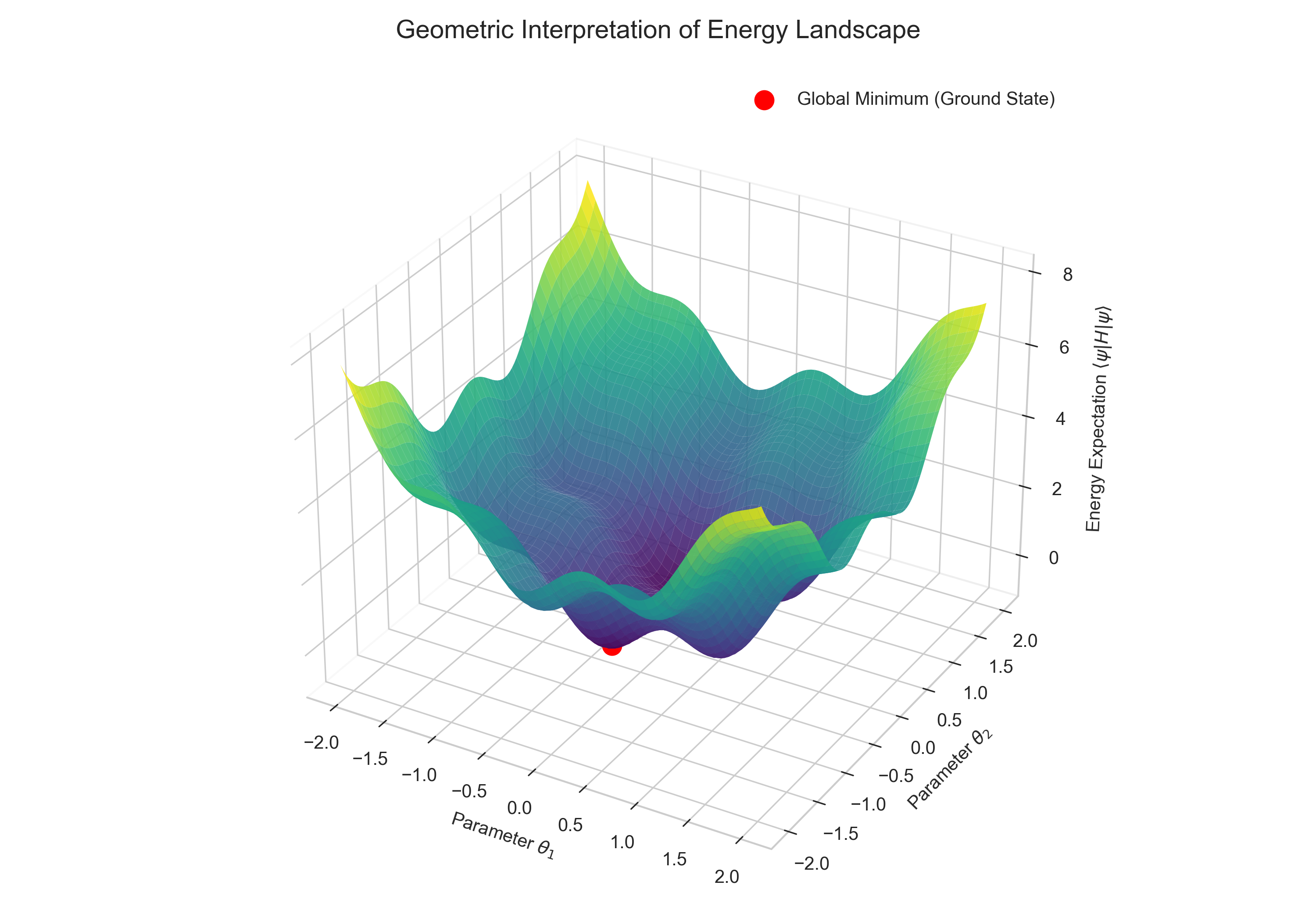
This brings us to a fundamental property known as the Variational Principle. It states that if you take any arbitrary normalized vector \(v\) and compute this product, the result will always be greater than or equal to the lowest eigenvalue:
\[v^T A v \ge \lambda_0\]
If you are interested in the mathematical rigor behind this principle, you can expand the section below for a step-by-step proof.
To prove that \(v^T A v \ge \lambda_0\), we rely on the Spectral Theorem. Since \(A\) represents a physical observable (like a Hamiltonian), it is a Hermitian matrix. This guarantees two things:
- All its eigenvalues \(\lambda_i\) are real.
- Its eigenvectors \(\{x_0, x_1, \dots, x_{n-1}\}\) form a complete orthonormal basis.
Let’s order the eigenvalues such that \(\lambda_0 \le \lambda_1 \le \dots \le \lambda_{n-1}\).
Since the eigenvectors form a basis, any arbitrary vector \(v\) can be written as a linear combination of these eigenvectors:
\[v = \sum_{i} c_i x_i\]
Because \(v\) is normalized (\(v^T v = 1\)) and the basis is orthonormal (\(x_i^T x_j = \delta_{ij}\)), the sum of the squared coefficients must equal 1:
\[\sum_{i} |c_i|^2 = 1\]
Now, let’s look at the action of \(A\) on this expansion:
\[A v = A \left( \sum_{i} c_i x_i \right) = \sum_{i} c_i (A x_i) = \sum_{i} c_i \lambda_i x_i\]
Next, we calculate the expectation value \(v^T A v\):
\[v^T A v = \left( \sum_{j} c_j x_j \right)^T \left( \sum_{i} c_i \lambda_i x_i \right)\]
Due to the orthonormality of the eigenvectors (the product \(x_j^T x_i\) is 1 if \(i=j\) and 0 otherwise), the cross-terms vanish, leaving us with a weighted sum of the eigenvalues:
\[v^T A v = \sum_{i} |c_i|^2 \lambda_i\]
Here is the crucial step. Since \(\lambda_0\) is the smallest eigenvalue, we know that \(\lambda_i \ge \lambda_0\) for all \(i\). Therefore, we can replace \(\lambda_i\) with \(\lambda_0\) to form an inequality:
\[\sum_{i} |c_i|^2 \lambda_i \ge \sum_{i} |c_i|^2 \lambda_0\]
We can factor out \(\lambda_0\):
\[v^T A v \ge \lambda_0 \left( \sum_{i} |c_i|^2 \right)\]
Since \(\sum |c_i|^2 = 1\), the proof is complete:
\[v^T A v \ge \lambda_0\]
Turning Algebra into Optimization
This inequality gives us a clear strategy. To find the lowest eigenvalue, we don’t need to analytically solve the matrix equation. Instead, we can treat it as a minimization game: we need to try different vectors \(v\) until we find the one that produces the lowest possible value for \(v^T A v\).
However, trying vectors blindly is not efficient. The vector space is simply too vast. To make this manageable, we transform the search into an optimization problem.
Instead of picking random vectors, we construct a vector that depends on a set of tunable scalar parameters. Let’s say we have a problem with \(n\) dimensions; theoretically, we need at most \(n\) parameters to explore the space. We can denote this parameterized vector as \(v(\theta)\). By tweaking these \(\theta\) parameters, we navigate the vector space, searching for the minimum value.
The Complexity Barrier and the Quantum Solution
This sounds straightforward enough to handle classically, so why do we need a quantum computer?
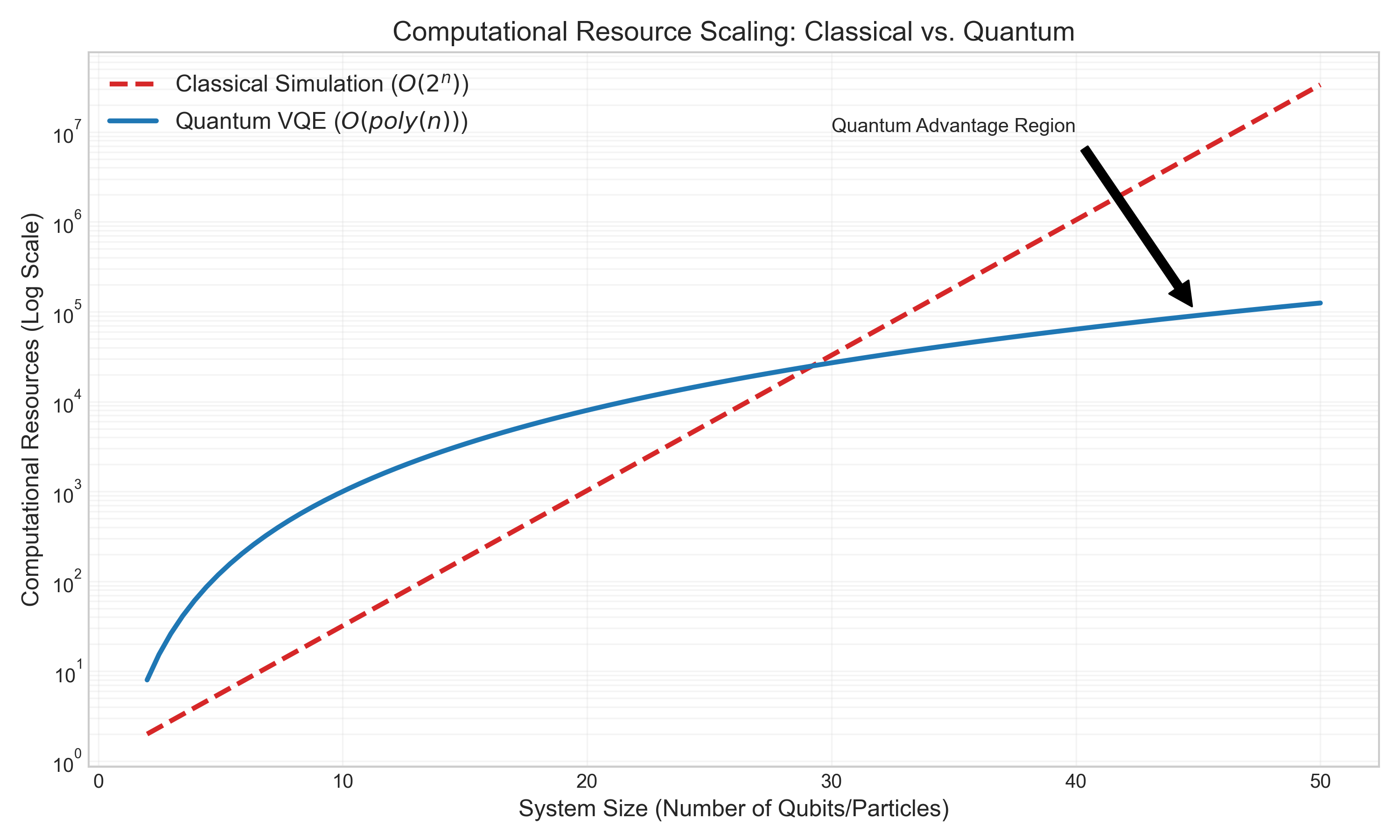
The problem lies in the complexity. As the system we are studying grows (for example, adding more atoms to a molecule), the dimension of the matrix \(A\) explodes exponentially. For a system that is still relatively small in physical terms, the vector \(v\) becomes so large that a classical supercomputer cannot even store it, let alone perform the matrix multiplications required to calculate \(v^T A v\).
The chart below illustrates this dramatic difference in scaling. While classical resources grow exponentially, a quantum algorithm like VQE offers a much more favorable polynomial scaling.
This is where the quantum connection is made. In quantum mechanics, the expression \(v^T A v\) is written using Dirac notation as:
\[\langle v | A | v \rangle\]
This is known as the quantum expectation value.
While calculating this is a choking point for classical computers, it is a native operation for a quantum computer. We can prepare the state \(|v\rangle\) on a quantum processor and measure the expectation value of the operator \(A\) directly. This allows us to evaluate our “cost function” efficiently, while a classical computer handles the task of updating the parameters \(\theta\) to drive us toward the solution.
Next Steps: In my next post, I will dive into the implementation details: specifically, how we efficiently create these parameterized vectors (the ansatz - German for ‘approach’ or ‘trial’) on actual quantum hardware, and the precise circuits required to measure the quantum expectation value \(\langle v | A | v \rangle\).